


Our test base for Power extends on the one of [2]. Most of our tests are produced by one of the generators of the diy tool suite from cycles of candidate relaxations, a concise and precise mean to describe violations of sequential consistency, and thus relevant tests for memory model testing. For instance, by listing critical cycles of size four, we get all the six basic violations of sequential consistency on two threads: 2+2W, LB, MP, R, S and SB. See the Quick reference for litmus test families for more such tests up to four threads.
Additional tests are:
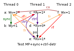
Detours are relevant to this work as they occur in the model definition. Moreover, test MP+sync+ctrl-detr unveiled a bug in the model of [3].
The ARM test set is broadly similar, considering that ARM fences are different. We considered ARM dsb and dmb fences, and their variations dsb.st and dmb.st.
Finally our test set for Power power-tests.tgz totals 8121 tests; while our test set for ARM arm-tests.tgz totals 9763 tests.
The purpose of this document is to illustrate the companion paper. We do so by the means of tables. Nevertheless, we also provide model ouputs, complete logs of our experiments, and test validation summaries.
Tests are of course programs that we either simulate or run on actual hardware. As a result of those runs, we collect the final values of some observed locations, either local (i.e. registers) or global (i.e. memory cells). Observed locations can be given explicitly in test source but more often they derive from a given final condition, a quantified boolean proposition that appears at the end of test source. In turn, an existential test condition identifies one of several executions of a given test. As described in Sec. 3 of the paper, an execution is a set of events (memory accesses, fences and branch events), plus a few relations: program order po, and communication relations read-from rf and coherence order co (plus some other relations such as dependencies or the from-read relation fr which derive from the basic ones).
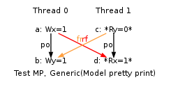
In effect, when we describe tests we more often describe test executions than plain programs. For instance, the web page for the MP test not only gives the program (and final condition) as given by test source, but also diagram(s) of execution as the following one that here describes the non-SC (non Sequentially Consistent) execution of the MP test:
Executions for behaviour:
"1:r1=1 ; 1:r3=0"
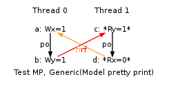
This diagram derives from the final condition that identifies the situation when Thread 1 loads value 1 from location y and then the value 0 from location x.
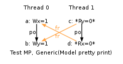
Notice that by changing the final condition of tests we get others executions. For instance, we get the SC executions of MP as:
PPC MP
{
0:r2=x; 0:r4=y;
1:r2=y; 1:r4=x;
}
 P0           | P1           ;
 li r1,1      | lwz r1,0(r2) ;
 stw r1,0(r2) | lwz r3,0(r4) ;
 li r3,1      |              ;
 stw r3,0(r4) |              ;
(* Was exists (1:r1=1 \/ 1:r3=0) *)
exists (1:r1=1 /\ 1:r3=1) \/ (1:r1=0 /\ 1:r3=0) \/  (1:r1=0 /\ 1:r3=1)
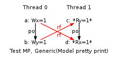
That is, we changed the final condition of MP to a new one that lists the final values of the test when run on the SC model. This results in the following three execution diagrams:
Executions for behaviour:
"1:r1=0 ; 1:r3=0"
Executions for behaviour:
"1:r1=0 ; 1:r3=1"
Executions for behaviour:
"1:r1=1 ; 1:r3=1"
It is worth noticing that a given set of final values for all observed locations may cover more than one execution. For instance consider LB+data-pos+pos-data, a variation of of LB:
PPC LB+data-pos+pos-data
{
0:r2=x; 0:r4=y;
1:r2=y; 1:r5=x;
}
 P0           | P1           ;
 lwz r1,0(r2) | lwz r1,0(r2) ;
 xor r3,r1,r1 | lwz r3,0(r2) ;
 addi r3,r3,1 | xor r4,r3,r3 ;
 stw r3,0(r4) | addi r4,r4,1 ;
 li r5,2      | stw r4,0(r5) ;
 stw r5,0(r4) |              ;
exists
(y=2 /\ 0:r1=1 /\ 1:r1=1)
By observing the final values of registers 0:r1 and 1:r1, the above final condition targets some LB style non-SC execution a → b → d → f, or more precisely:
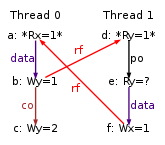
But the register 1:r3 (second load of y by Thread 1) has to get its value either from the initial value 0 of y, or from the stores to y by Thread 0 (b or c). This results in the following three executions:
Executions for behaviour:
"0:r1=1 ; 1:r1=1 ; y=2"
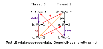
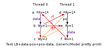
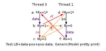
Notice that, in the above LB+data-pos+pos-data example, the ambiguity in executions results from not observing the register 1:r3. Unfortunately many of our tests present such a lack of observation. To reveal that situation in execution diagram, we picture observed reads between two stars ’*’. For instance, in the above diagrams the first memory load by Thread 1 is written “d:*Ry=1* ”, while the second memory load is written “e:Ry=0”,“e:Ry=1”, and “e:Ry=2”.
Another source of ambiguity originates from tests that feature three stores or more to the same location. Consider the simple test 3W:
PPC 3W
{
0:r2=x; 1:r2=x; 2:r2=x;
}
 P0           | P1           | P2           ;
 li r1,1      | li r1,2      | li r1,3      ;
 stw r1,0(r2) | stw r1,0(r2) | stw r1,0(r2) ;
exists (x=3)
This tests consists in three threads each of which performs a store to the global location x. The final condition x=3 does not characterise an unique coherence order: as the two orders a → b → c and b → a → c admit the store of value 3 as their last element.
Such ambiguity can be avoided by adding an extra thread to the test. The new thread’s sole purpose is to read x three times, saving the loaded values in registers that are observed, see test 3W+OBS. We seldom use this possibility as such an observation of coherence orders requires sheer luck to perform well during hardware experiments. An alternative is to add some memory loads to the test threads themselves, as in test 3W+OBS-LOCAL. Unfortunately, this latter technique clutters execution diagrams, which become barely readable, saved for the most simple tests. Besides, those techniques assume that the tested system does not permit loads to contradict the coherence order. In our words, the tested system must obey the sc per location check.