Memory models and the cat languageThe herdtools7 team |
This tutorial is an introduction to
herdtools (release seven).
It mainly focuses on the simulator herd.
However the last part briefly addresses the test generators
diyone and diycross, as well as litmus,
a tool for running tests on hardware.
Readers that wish to go beyond this introduction
can refer to herdtools
documentation.
Before starting
Please follow the the software installation instructions.
In a fresh directory, download the archive kit.tgz and unpack
it with command tar zxmf kit.tgz. You now have all
the necessary files at hand.
1 Using herd
We first consider a simple “message passing” test
MP:
AArch64 MP
{
int x=0;
int y=0;
0:X1=x; 0:X3=y;
1:X0=y; 1:X2=x;
}
 P0          | P1          ;
 MOV W0,#1   | LDR W1,[X0] ;
 STR W0,[X1] | LDR W3,[X2] ;
 MOV W2,#1   |             ;
 STR W2,[X3] |             ;
exists (1:X1=1 /\ 1:X3=0)
The test is written in AArch64 (Armv8) assembly, it consists of two threads
P0 and P1 and operates on two memory locations x
and y. The memory location values are 0 initially, while the two
threads do the following:
Overview of how herd works
An execution essentially consists of a set of Effects such as
writes and reads to and from memory (viz, Memory Write Effects and Memory Read
Effects), equipped with relations such as the program order po
which lifts the order in which program statements are written to Effects, and
the communication relations:
- The Reads-from relation
rf that relates a Memory Write
Effect w to the Memory Read Effects that read the value written
by w. Notice that the inverse of rf, written
rf^-1, is a function.
- The Coherence order(s)
co that orders the
writes to the same memory location. This means that if you were sitting in a memory location like this little elf, you would see writes falling one by one onto you.
| |  | |
| Wx0 —→co Wx1 —→co | x=2 | —→co Wx3 —→co ⋯
|
- The From-read relation
fr that relates a Memory Read
Effect r to the Memory Write Effects that overwrite its location. The
fr relation is computed from the previous two relations
as: let fr = rf^-1; co. In other words,(r,w)
∈ rf when w strictly follows the write that feeds
r in the Coherence order of their location.
The herd tool first enumerates all possible executions, by
matching writes with reads in all possible manners, i.e. by
enumeratimg possible rf relations; and by ordering all
writes to the same location in all possible manners, i.e. by
enumerating possible co relations. It then filters those
execution candidates according to a memory model given as a
cat file.
Using herd
By using the following model empty.cat
Empty
// Define the coherence (co) relation
include "cos.cat"
(which is empty in the sense that it does not impose any ordering constraints
on Reads-from and Coherence order) we enumerate all possible execution
candidates:
% herd7 -cat empty.cat MP.litmus
Test MP Allowed
States 4
1:X1=0; 1:X3=0;
1:X1=0; 1:X3=1;
1:X1=1; 1:X3=0;
1:X1=1; 1:X3=1;
Ok
Witnesses
Positive: 1 Negative: 3
Condition exists (1:X1=1 /\ 1:X3=0)
Observation MP Sometimes 1 3
Time MP 0.01
Hash=4af4ac4effa358424acf380711d0da64
In the output above, there are four (one “positive” and three
“negative”) execution candidates, of which one
satisfies the final condtion exists 1:X1=1 /\ 1:X3=0.
Those four executions also manifest themselves
as four different final states that result from the two possible
rf choices: either read the initial value 0 or the value 1
written by P0, for the two locations x and y.
Those choices of rf are made apparent in the
execution candidates:
Some of the images display fr relations from some reads of
P1 to some writes of P0. This
situation results from the reads reading the initial values or,
equivalently, reading from initial writes (which we have not displayed here).
Initial writes always precede
the writes to the same location performed by the test code.
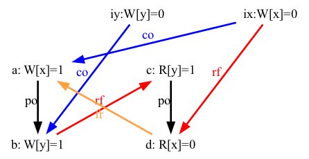
The following image details this situation, with initial writes displayed:
In the picture above, we now clearly see that the read d reads from the initial write ix, which is coherence-before the write a, in other words:
With the graphiz tools and the PostScript viewer
gv installed one can display those images by using the
configuration file show.cfg:
% herd7 -conf show.cfg -cat empty.cat -show all -gv MP.litmus
Alternatively and provided graphviz is installed,
one can produce four PDF images by using the shell script
img.sh as follows:
% herd7 -conf show.cfg -cat empty.cat -show all -o . MP.litmus
% sh ./img.sh MP.dot
We can then display the images with the appropriate PDF viewer.
For instance, on an Apple computer:
% open MP-0?.pdf
Question
Run herd on the following R test
with the empty model.
AArch64 R
{
int x=0;
int y=0;
0:X1=x; 0:X3=y;
1:X1=y; 1:X2=x;
}
 P0          | P1          ;
 MOV W0,#1   | MOV W0,#2   ;
 STR W0,[X1] | STR W0,[X1] ;
 MOV W2,#1   | LDR W3,[X2] ;
 STR W2,[X3] |             ;
exists ([y]=2 /\ 1:X3=0)
Count execution candidates and explain the result in terms of rf and
co enumeration.
If you have the required software installed, show the corresponding images.
2 Sequential consistency, sequential consistency per location
Sequential consistency (SC) was defined by Leslie Lamport as an
execution model for concurrent, multi-threaded programs. In SC,
program executions are interleavings of the program order of
instructions on each thread.
Defining SC
We first give sc.cat, the SC model in cat:
"SC model"
// Define the coherence (co) relation
include "cos.cat"
// Communication relations
let com = rf|co|fr
// Consistency condition for SC
acyclic po|com as SC
That is, the model acccepts execution candidates, such that the union
(“|”) of the program order (po) and of the
communication relations (rf|co|fr) is
an acyclic relation. Or, equivalently, cycles in the union of program
order and of the communication relations are forbidden.
Question
Show that the original SC formulation and this cat one are equivalent.
Testing SC
We now consider a series of six tests that illustrates sequential consistency
on two threads and two memory locations:
2+2WAArch64 2+2W
{
0:X1=x; 0:X3=y;
1:X1=y; 1:X3=x;
}
P0 | P1 ;
MOV W0,#2 | MOV W0,#2 ;
STR W0,[X1] | STR W0,[X1] ;
MOV W2,#1 | MOV W2,#1 ;
STR W2,[X3] | STR W2,[X3] ;
exists ([x]=2 /\ [y]=2)
| | LBAArch64 LB
{
0:X0=x; 0:X3=y;
1:X0=y; 1:X3=x;
}
P0 | P1 ;
LDR W1,[X0] | LDR W1,[X0] ;
MOV W2,#1 | MOV W2,#1 ;
STR W2,[X3] | STR W2,[X3] ;
exists (0:X1=1 /\ 1:X1=1)
| | MPAArch64 MP
{
0:X1=x; 0:X3=y;
1:X0=y; 1:X2=x;
}
P0 | P1 ;
MOV W0,#1 | LDR W1,[X0] ;
STR W0,[X1] | LDR W3,[X2] ;
MOV W2,#1 | ;
STR W2,[X3] | ;
exists (1:X1=1 /\ 1:X3=0)
|
RAArch64 R
{
0:X1=x; 0:X3=y;
1:X1=y; 1:X2=x;
}
P0 | P1 ;
MOV W0,#1 | MOV W0,#2 ;
STR W0,[X1] | STR W0,[X1] ;
MOV W2,#1 | LDR W3,[X2] ;
STR W2,[X3] | ;
exists ([y]=2 /\ 1:X3=0)
| | SBAArch64 SB
{
0:X1=x; 0:X2=y;
1:X1=y; 1:X2=x;
}
P0 | P1 ;
MOV W0,#1 | MOV W0,#1 ;
STR W0,[X1] | STR W0,[X1] ;
LDR W3,[X2] | LDR W3,[X2] ;
exists (0:X3=0 /\ 1:X3=0)
| | SAArch64 S
{
0:X1=x; 0:X3=y;
1:X0=y; 1:X3=x;
}
P0 | P1 ;
MOV W0,#2 | LDR W1,[X0] ;
STR W0,[X1] | MOV W2,#1 ;
MOV W2,#1 | STR W2,[X3] ;
STR W2,[X3] | ;
exists ([x]=2 /\ 1:X1=1)
|
We may observe that those tests all have a final condition with an
existential quantifier. We say that a model allows a test when running
the test on top of the model yieds at least an outcome that satisfies
the final condition. Otherwise, the model forbids the test, or the test
is a violation of the model.
As we shall see, the final condition of the six basic tests
each characterise a certain violation of the SC model.
The source of these tests are in the sub-directory
sc-tests/. The directory also contains the index
file sc-tests/@all, so that one can run all the tests on top
of the empty and SC models as:
% herd7 -cat ./empty.cat sc-tests/@all > EM
% herd7 -cat ./sc.cat sc-tests/@all > SC
We can now compare the two models on the test base:
% mcompare7 -show v EM SC
   |Kind | EM SC
-----------------
-----------------
2+2W|Allow| Ok No
-----------------
LB  |Allow| Ok No
-----------------
MP  |Allow| Ok No
-----------------
R   |Allow| Ok No
-----------------
S   |Allow| Ok No
-----------------
SB  |Allow| Ok No
-----------------
We see that the empty model allows all tests (which is not surprising), while
the SC model forbids all tests. Namely, each of the six corresponding
execution candidates exhibits an SC cycle:
Have a go at producing and displaying those images:
% herd7 -cat empty.cat -conf show.cfg -show prop -gv sc-tests/@all
On MacOS, try using option -preview instead of -gv.
It is important to notice that we use option -show prop and
not -show all. As a consequence, only the executions that
validate the final condition are displayed.
Question
When given no command line option -cat name.cat,
herd uses the default model of the test architecture —
here aarch64.cat from the herd distribution.
How does the model aarch64.cat
behave on the six basic tests? Notice that herd somehow
verbose output contains a summary of observations introduced by the
keyword “Observation”.
Writing a SC-per-location model
A very important property of most memory models we know of is
SC-per-location. As its name suggests, the property amounts to SC
applied to each memory location individually.
Consider the following test test MP+READ:
AArch64 MP+READ
{
 0:X1=x; 0:X3=y;
 1:X0=y; 1:X2=x;
}
 P0          | P1          ;
 MOV W0,#1   | LDR W1,[X0] ;
 STR W0,[X1] | LDR W3,[X2] ;
 MOV W2,#1   | LDR W5,[X0] ;
 STR W2,[X3] |             ;
exists 1:X1=1 /\ 1:X3=0 /\ 1:X5=0
The test is the MP test with an additional read of y at the end of P1.
The following execution of MP+READ is forbidden by SC
but allowed by SC-per-location:
Namely, the execution contains the following SC cycle: a:W[x]1 → b:W[y]1 → c:R[y]1 → d:R[x]0 → a:⋯
As a consequence the displayed execution is forbidden by SC. However, the Effects a and b operate on different locations and, as the cycle is the only one, the execution is allowed by the SC-per-location model.
By contrast, the following execution is forbidden by both models:
Namely, there is now an additional SC cycle: b:W[y]1 →
c:R[y]1 → e:R[y]0 → b:⋯, which suffices for
the SC-per-location model to forbid the execution, as all Effects in
cycle operate on the same location y.
Question
Starting from the model sc.cat, write a new cat file
sc-loc.cat that implements the SC-per-location model. The model
sc-loc.cat must forbid the test MP+READ and all the tests in
the coherence-tests/ sub-directory.
As a check, the following command should yield no output at all.
% herd7 -cat sc-loc.cat MP+READ.litmus coherence-tests/*.litmus | grep Sometimes
As a more demanding check, one can compare model output with
the reference file SC-LOC-REF.txt:
% herd7 -cat sc-loc.cat @sc-loc > SC-LOC.txt
% mcompare7 SC-LOC-REF.txt SC-LOC.txt
A little help:
The tool herd pre-defines the relation loc that relates
Effects operating on the same location and implements the usual
operators on relations (See
herd manual).
More help.
2.1 Alternative formulation
One can show
that the SC-per-location condition is equivalent to the property
which ensures that the transitive closure of communications does not contradict
the program order.
By definition, two relations r1 and r2 contradict each other
when r1 relates e1 to e2 while r2 relates e2 to e1.
| ∃ e1, e2, (e1,e2) ∈ r1 and (e2,e1)
∈ r2.
|
In other words, the sequence of r1 and r2 is reflexive. In cat,
we can make sure that r1 and r2 do not contradict each other as follows:
irreflexive r1; r2
Where “;” is the sequence operator.
Question
From the observation above, write an alternative
SC-per-location model as the cat file sc-loc-bis.cat. One
can check whether sc-loc-bis.cat indeed implements the
SC-per-location model by using the tool mcompare.
% herd7 -cat sc-loc-bis.cat @sc-loc > SC-LOC-BIS.txt
% mcompare7 SC-LOC-REF.txt SC-LOC-BIS.txt
Some help:
The postfix operator “+” computes
the transitive closure of a
relation r0 (let r = r0+). One
can also proceed by a recursive definition:
let rec r = r0 | r;r.
3 TSO and beyond
Take a detour to explore some features of the ARM memory model before
testing your machine. Maybe your computer is “TSO and beyond”.
4 Test your machine
Some simple tests
The herdtools toolbox contains test generators. All generators
follow the same principle of generating tests from (SC-)cycles.
Cycles wil be represented by lists of edges.
For instance, here is again the picture of the test MP:
The cycle above can be expressed as “PodWW Rfe PodRR FRe”,
where PodWW (resp. PodRR) is “program order from write to write, changing location” (resp. read to read), Rfe and Fre and the external rfe and fre communication relations.
When clear from context the “W” and “R” specifiers can be replaced by a wildcard “*”. One benefit of the cycle notation resides in its generality. In the example below, we generate two tests MP for the AArch64 and X86_64 architecture, and one for the C language,
by using the tool diyone that takes a cycle as argument and
outputs the corresponding test.
diyone7 -arch AArch64 Pod** Rfe Pod** Fre
AArch64 A
{
0:X1=x; 0:X3=y;
1:X0=y; 1:X2=x;
}
 P0          | P1          ;
 MOV W0,#1   | LDR W1,[X0] ;
 STR W0,[X1] | LDR W3,[X2] ;
 MOV W2,#1   |             ;
 STR W2,[X3] |             ;
exists (1:X1=1 /\ 1:X3=0)
| | % diyone7 -arch X86_64 Pod** Rfe Pod** Fre
X86_64 A
{
}
P0 | P1 ;
movl $1,(x) | movl (y),%eax ;
movl $1,(y) | movl (x),%ebx ;
exists (1:rax=1 /\ 1:rbx=0)
| | % diyone7 -arch C Pod** Rfe Pod** Fre
C A
{}
P0 (volatile int* y,volatile int* x) {
*x = 1;
*y = 1;
}
P1 (volatile int* y,volatile int* x) {
int r0 = *y;
int r1 = *x;
}
exists (1:r0=1 /\ 1:r1=0)
|
Another generator, diycross produces several tests where
diyone produces one. The tool diycross takes a list
of edge sets, where diyone takes a list of edges.
Then, diycross enumerate all cycles built by selecting one
edge from every edge set.
A typical invocation of diycross is:
% diycross7 -arch Arch Pod** Rfe,Fre,Coe Pod** Rfe,Fre,Coe
Generator produced 6 tests
Where Coe is the external coherence relation coe and
Arch is one of the architectures that
herdtools implements.
The edge sets are comma-separated lists of edges and wildcards are expanded
—
Pod** expands to PodWW,PodWR,PodRW,PodRR.
Valid cycles obey some consistency constraints.
In particular, successive edges have to agree on their
common point to be either a read or a write.
For instance, PodRR can be followed by
Fre, not by Coe, nor by Rfe which both
start with a “W”.
Finally the cycle list specification
“Pod** Rfe,Fre,Coe Pod** Rfe,Fre,Coe”
expands to the six “basic” cycles:
2+2W: PodWW Coe PodWW Coe LB: PodRW Rfe PodRW Rfe MP: PodWW Rfe PodRR Fre SB: PodWR Fre PodWR Fre R: PodWW Coe PodWR Fre S: PodWW Rfe PodRW Coe
And diycross generates the six “basic” tests, with
their appropriate final condition that characterises the cyclic
execution.
Question
In a fresh directory, generate the following generalisation of the
basic tests: Pod** edges can remain or be replaced by full-fence
edges Fenced**.
Generate tests for the architecture of your machine — most likely
X86_64 or AArch64.
Running the tests
Now we run the tests with litmus.
The tool litmus has many options and several operating modes,
described in the
documentation.
Basically, the tool consumes litmus tests and produces C sources files that
can be compiled and executed.
In particular, litmus adds code
that interfaces the test with the operating system, collects and outputs
results etc.
We limit ourselves to a simple, local, compile-and-execute process.
For the process to apply, your machine should have gcc installed
(command line tools installed for MacOS).
It is convenient to store the C source files in yet another
directory, say R/.
% mkdir -p R
Most of the appropriate options are from a configuration file. Here is
a possible comand line for an Intel-based Linux machine:
% litmus7 -mach x86_64 -a 2 -o R @all
The command-line option “-a 2” limits the number of cores devoted
to tests, one can give a higher number if adequate.
For a ARMv8 based Apple computer, try:
% litmus7 -mach M1 -a 2 -o R @all
Then, enter the R/ directory, compile and run the tests:
% cd R
% make -j 2 #Or more.
% sh ./run.sh > LOG.txt
If your machine is neither an Intel based Linux machine, nor a recent
Apple machine, please ask someone.
Question
Run the tests, so as to
answer the following questions about the memory model
of your machine.
- Is my machine memory model sequential consistency (SC)?
- Can my machine memory model be TSO?
- If my machine is not SC. Do experiments suggest
that full-fences suffice to restore SC?
This document was translated from LATEX by
HEVEA.