Part III |
The tool herd7 is a memory model simulator. Users may write simple, single events, axiomatic models of their own and run litmus tests on top of their model. The herd7 distribution already includes some models.
The authors of herd7 are Jade Alglave and Luc Maranget.
This section introduces cat, our language for describing memory models. The cat language is a domain specific language for writing and executing memory models. From the language perspective, cat is loosely inspired by OCaml. That is, it is a functional language, with similar syntax and constructs. The basic values of cat are sets of events, which include memory events but also additional events such as fence events, and relations over events.
The simulator herd7 accepts models written in text files. For instance here is sc.cat, the definition of the sequentially consistent (SC) model in the partial-order style:
SC

include "fences.cat"
include "cos.cat"

(* Atomic *)
empty rmw & (fre;coe) as atom

(* Sequential consistency *)
show sm\id as si
acyclic po | ((fr | rf | co);sm) as sc
The model above illustrates some features of model definitions:
SC), which can also be a
string (in double quotes) in case the tag includes special characters or spaces.
po (program order)
and rf (read from) are pre-defined.
The remaining two communication relations (co and fr)
are computed by the included file cos.cat, which we describe later
— See Sec. 14.4.
For simplicity, we may as well assume that co
and fr are pre-defined.
let construct.
Here, a new relation com is the union “|” of
the three pre-defined communication relations.
po | com”
(i.e. the union of program order po and of communication
relations) is required to be acyclic.
Checks can be given names by suffixing them with
“as name”.
This last feature will be used in Sec. 15.2
One can then run some litmus test, for instance SB (for Store Buffering, see also Sec. 1.1), on top of the SC model:
% herd7 -model ./sc.cat SB.litmus
Test SB Allowed
States 3
0:EAX=0; 1:EAX=1;
0:EAX=1; 1:EAX=0;
0:EAX=1; 1:EAX=1;
No
Witnesses
Positive: 0 Negative: 3
Condition exists (0:EAX=0 /\ 1:EAX=0)
Observation SB Never 0 3
Hash=7dbd6b8e6dd4abc2ef3d48b0376fb2e3
The output of herd7 mainly consists in
the list of final states that are allowed by the simulated model.
Additional output relates to the test condition.
One sees that the test condition does not validate on top of SC,
as “No” appears just after the list of final states
and as there is no “Positive” witness.
Namely, the condition “exists (0:EAX=0 /\ 1:EAX=0)”
reflects a non-SC behaviour, see Sec. 14.1.
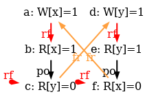
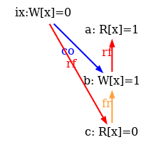
The simulator herd7 works by generating all candidate executions of a given test. By “candidate execution” we mean a choice of events, program order po, of the read-from relation rf and of final writes to memory (last write to a given location)6. In the case of the SB example, we get the following four executions:
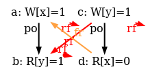
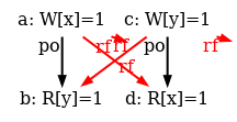
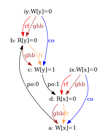
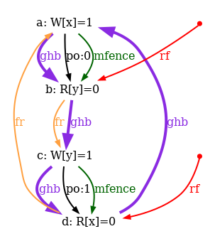
Indeed, there is no choice for the program order po, as there are no conditional jumps in this example; and no choice for the final writes either, as there is only one store per location, which must be co-after the initial stores (pictured as small red dots). Then, there are two read events from locations x and y respectively, which take their values either from the initial stores or from the stores in program. As a result, there are four possible executions. The model sc.cat gets executed on each of the four candidate executions. The three first executions are accepted and the last one is rejected, as it presents a cycle in po | fr. On the following diagram, the cycle is obvious:
However, the non-SC execution shows up on x86 machines, whose memory model is TSO. As TSO relaxes the write-to-read order, we attempt to write a TSO model tso-00.cat, by simply removing write-to-read pairs from the acyclicity check:
"A first attempt for TSO"

include "cos.cat"

(* Communication relations that order events*)
let com-tso = rf | co | fr
(* Program order that orders events *)
let po-tso = po & (W*W | R*M)

(* TSO global-happens-before *)
let ghb = po-tso | com-tso
acyclic ghb as tso
show ghb
This model illustrates several features of model definitions:
W, R and M, which are
the sets of write events, read events and of memory events, respectively.
*” that returns the cartesian
product of two event sets as a relation.
&” that operates on sets and
relations.
As a result, the effect of the declaration
let po-tso = po & (W*W | R*M) is to define po-tso
as the program order on memory events minus write-to-read pairs.
We run SB on top of the tentative TSO model:
% herd7 -model tso-00.cat SB.litmus
Test SB Allowed
States 4
0:EAX=0; 1:EAX=0;
0:EAX=0; 1:EAX=1;
0:EAX=1; 1:EAX=0;
0:EAX=1; 1:EAX=1;
Ok
Witnesses
Positive: 1 Negative: 3
...
The non-SC behaviour is now accepted, as write-to-read po-pairs
do not participate to the acyclicity check any more. In effect, this allows
the last execution above,
as ghb (i.e.
po-tso | com-tso) is acyclic.
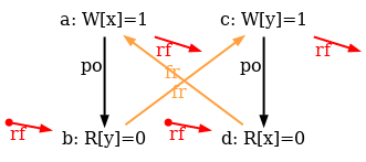
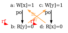
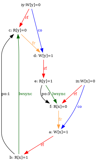
However, our model tso-00.cat is flawed: it is still to strict, forbidding some behaviours that the TSO model should accept. Consider the test SB+rfi-pos, which is test STFW-PPC for X86 from Sec. 1.3 with a normalised name (see Sec. 12.1). This test targets the following execution:
Namely the test condition
exists (0:EAX=1 /\ 0:EBX=0 /\ 1:EAX=1 /\ 1:EBX=0)
specifies that Thread 0 writes 1 into location x,
reads the value 1 from the location x (possibly by store forwarding) and
then reads the value 0 from the location y;
while Thread 1 writes 1 into y,
reads 1 from y and then reads 0 from x.
Hence, this test derives from the previous SB
by adding loads in the middle, those loads
being satisfied from local stores.
As can be seen by running the test on top of the tso-00.cat
model, the target execution is forbidden:
% herd7 -model tso-00.cat SB+rfi-pos.litmus
Test SB+rfi-pos Allowed
States 15
0:EAX=0; 0:EBX=0; 1:EAX=0; 1:EBX=0;
...
0:EAX=1; 0:EBX=1; 1:EAX=1; 1:EBX=1;
No
Witnesses
Positive: 0 Negative: 15
..
However, running the test with litmus demonstrates that the behaviour is observed on some X86 machine:
% arch
x86_64
% litmus7 -mach x86 SB+rfi-pos.litmus
...
Test SB+rfi-pos Allowed
Histogram (4 states)
11589 *>0:EAX=1; 0:EBX=0; 1:EAX=1; 1:EBX=0;
3993715:>0:EAX=1; 0:EBX=1; 1:EAX=1; 1:EBX=0;
3994308:>0:EAX=1; 0:EBX=0; 1:EAX=1; 1:EBX=1;
388   :>0:EAX=1; 0:EBX=1; 1:EAX=1; 1:EBX=1;
Ok

Witnesses
Positive: 11589, Negative: 7988411
Condition exists (0:EAX=1 /\ 0:EBX=0 /\ 1:EAX=1 /\ 1:EBX=0) is validated
...
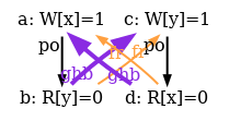
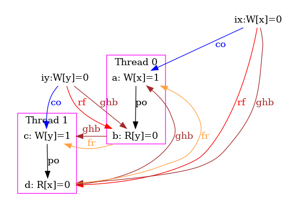
As a conclusion, our tentative TSO model is too strong. The following diagram pictures its ghb relation:
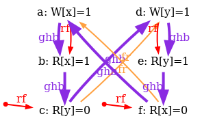
One easily sees that ghb is cyclic, whereas it should not. Namely, the internal read-from relation rfi does not create global order in the TSO model. Hence, rfi is not included in ghb. We rephrase our tentative TSO model, resulting into the new model tso-01.cat:
"A second attempt for TSO"

include "cos.cat"

(* Communication relations that order events*)
let com-tso = rfe | co | fr
(* Program order that orders events *)
let po-tso = po & (W*W | R*M)

(* TSP global-happens-before *)
let ghb = po-tso | com-tso
acyclic ghb
show ghb
As can be observed above rfi (internal read-from) is no longer included in ghb. However, rfe (external read-from) still is. Notice that rfe and rfi are pre-defined.
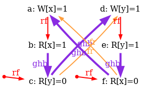
As intended, this new tentative TSO model allows the behaviour of test SB+rfi-pos:
%  herd7 -model tso-01.cat SB+rfi-pos.litmus
Test SB+rfi-pos Allowed
States 16
...
0:EAX=1; 0:EBX=1; 1:EAX=1; 1:EBX=0;
...
Ok
Witnesses
Positive: 1 Negative: 15
...
And indeed, the global-happens-before relation is no-longer cyclic:
We are not done yet, as our model is too weak in two aspects. First, it has no semantics for fences. As a result the test SB+mfences is allowed, whereas it should be forbidden, as this is the very purpose of the fence mfence.
One easily solves this issue by first defining the mfence
that relates events with a MFENCE event po-in-between them;
and then by adding mfence to the definition of po-tso:
let mfence = po & (_ * MFENCE) ; po
let po-tso = po & (W*W | R*M) | mfence
Notice how the relation mfence is defined from two pre-defined sets:
“_” the universal set of all events and MFENCE the set
of fence events generated by the X86 mfence instruction.
An alternative, more precise definition, is possible:
let mem-to-mfence = po & M * MFENCE
let mfence-to-mem = po & MFENCE * M
let mfence = mem-to-mfence; mfence-to-mem
This alternative definition of mfence, although yielding a smaller relation, is equivalent to the original one for our purpose of checking ghb acyclicity.
But the resulting model is still too weak, as it allows some behaviours that any model must reject for the sake of single thread correctness. The following test CoRWR illustrates the issue:
X86 CoRWR
{ }
 P0          ;
 MOV EAX,[x] ;
 MOV [x],$1  ;
 MOV EBX,[x] ;
exists (0:EAX=1 /\ 0:EBX=0)
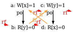
The test final condition targets the following execution candidate:
The TSO check “acyclic po-tso|com-tso” does not suffice to reject
two absurd behaviours pictured in the execution diagram above:
(1) the read a is allowed to
read from the po-after write b, as rfi is not included
in com-tso; and (2)
the read c is allowed to read the initial value of location x
although the initial write d is co-before the write b,
since po & (W * R) is not in po-tso.
For any model, we rule out those very
untimely behaviours by the so-called
uniproc
check that states that executions projected on events that access one variable
only are SC.
In practice, having defined po-loc as po restricted to
events that touch the same address (i.e.
as po & loc), we further require the acyclicity
of the relation po-loc|fr|rf|co.
In the TSO case, the uniproc check can be
somehow simplified by considering only
the cycles in po-loc|fr|rf|co that
are not already rejected by the main check of the model.
This amounts to design specific checks for the two relations that are
not global in TSO: rfi and po & (W*R).
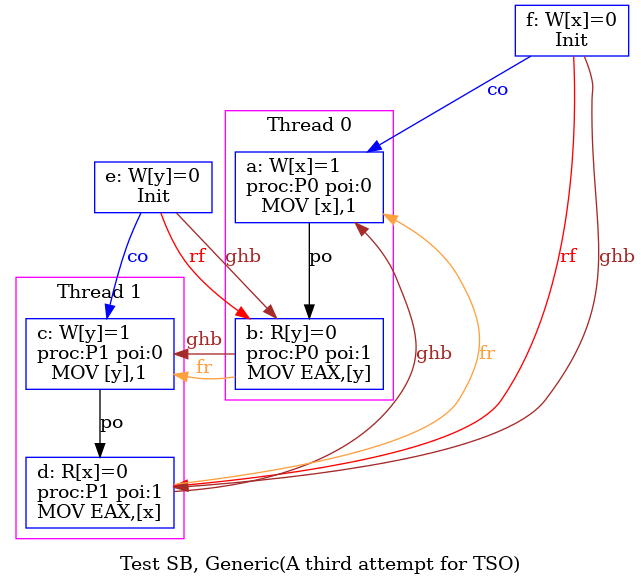
Doing so, we finally produce a correct model for TSO tso-02.cat:
"A third attempt for TSO"

include "cos.cat"

(* Uniproc check specialized for TSO *)
irreflexive po-loc & (R*W); rfi as uniprocRW
irreflexive po-loc & (W*R); fri as uniprocWR

(* Communication relations that order events*)
let com-tso = rfe | co | fr

(* Program order that orders events *)
let mfence = po & (_ * MFENCE) ; po
let po-tso = po & (W*W | R*M) | mfence

(* TSP global-happens-before *)
let ghb = po-tso | com-tso
show mfence,ghb
acyclic ghb as tso
This last model illustrates another feature of cat:
herd7 may also performs irreflexivity checks with the keyword
“irreflexive”.
We now illustrate another style of model.
We consider the original definition of sequential consistency [3].
An execution is SC when there exists a total (strict) order S on events such that:
po;
S-maximal write amongst those writes to location x
that S-precede r.
So we could just generate all total strict orders amongst events, and filter those “scheduling order candidates” according to the two rules above.
Things are a bit more complex in herd7, due to the presence of initial and final writes. Up to now we have ignored those writes, we are now going to integrate them explicitly.
Initial writes are write events that initialise the memory locations.
Initial writes are not generated by the instructions of the test.
Instead, they are created by herd7 machinery, and are available
from model text as the set IW.
Final writes may be generated by program instructions, and, when such,
they must be ordered by S.
A final write is a write to a phantom read performed once
program execution is over.
The constraint on final writes
originates from herd7 technique to enumerate execution candidates:
actual execution candidates also include a choice of final writes for
the locations that are observed in the test final condition7.
As test outcome (i.e. the final values of observed locations) is
settled before executing the model, it is important not to accept
executions that yield a different outcome. Doing so may validate outcomes
that should be rejected.
In practice, the final write wf
to location x must follow all other writes to x in S.
Considering that the set of final writes is available to cat models
as the pre-defined set FW,
the constraint on final writes
can be expressed as a relation:
let preSC = loc & (W \ FW) * FW
Where loc is a predefined relation that relates all events
that access the same location.
By contrast with final writes, initial writes are not generated by program instructions, and it is possible not to order them completely. In particular, it is not useful to order initial writes to different locations, nor the initial write to location x with any access to location y. Notice that we could include initial writes in S as we did for final writes. Not doing so will slightly improve efficiency.
Finally, the strict order S is not just any order on events,
it is a topological order of the events generated by threads
(implemented as the set ~IW. i.e. the complement of the set
of initial writes) that extends the pre-order preSC.
We can generate all such topological orders with the cat primitive
linearisations:
let allS = linearisations(~IW,preSC)
The call linearisations(E,r), where E is a set of events and r is a relation on events, returns the set of all total strict orders defined on E that extend r. Notice that if r is cyclic, the empty set is returned.
We now need to iterate over the set allS.
We do so with the with construct:
with S from allS
It is important to notice that the construct above extends the current execution candidate (i.e. a choice of events, plus a choice of two relations po and rf) with a candidate strict order S. In other words, the scope of the iteration is the remainder of the model text. Once model execution terminates for a choice of S (some element of allS), model execution restarts just after the with construct, with variable S bound to the next choice picked in allS.
As a first consistency check, we check that S includes the program order:
empty po \ S as PoCons
Notice that, to check for inclusion, we test the emptiness of relation
difference (operator “\”).
It remains to check that the rf relation of the execution candidate is the same as the one defined by condition 2. To that aim, we complement S with the constraint over initial writes that must precede all events to their location:
let S = S | loc & IW * (M \ IW)
Observe that S is no longer a total strict order. However, it is still a total strict order when restricted to events that access a given location, which is all that matters for condition 2 to give a value to all reads. As regards our SC model, we define rf-S the read-from relation induced by S as follows:
let WRS = W * R & S & loc  (* Writes from the past, same location *)
let rf-S = WRS \ (S;WRS)   (* Most recent amongst them *)
The definition is a two-step process: we first define
a relation WRS from writes to reads (to the same location)
that follow them in S. Observe that,
by complementing S with initial writes, we achieve that for any read r
there exists at least a write w such that (w,r) ∈ WRS.
It then remains to filter out non-maximal writes in WRS
as we do in the definition of rf-S, by the means of
the difference operator “\”.
We then check the equality of rf (pre-defined as part of the candidate
execution) and of rf-S by double inclusion:
empty rf \ rf-S as RfCons
empty rf-S \ rf as RfCons
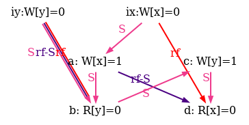
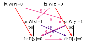
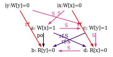
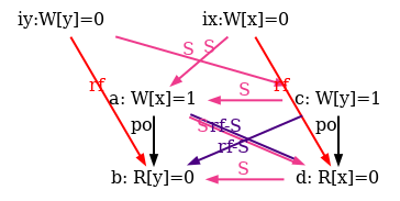
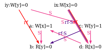
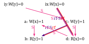
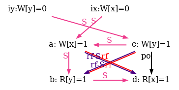
As an example, he show six attempts of po compatible S orders for the non-SC outcome of the test SB in figure 5.
Observe that all attempts fail as rf and rf-S are different in all diagrams.
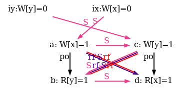
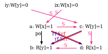
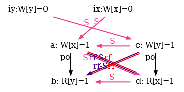
We also show all successful SC scheduling in figure 6.
Figure 6: SC executions of test SB. 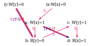
For reference we provide our complete model lamport.cat
"SC, L. Lamport style"

(* writes to location x precede final write to location x *)
let preSC =  loc & (W \ FW) * FW

(* Compute the set of total orders that extend preSC on program events *)
let allS = linearisations(~IW,preSC)

(* For all such orders *)
with S from allS

(* Check compatibility with po *)
empty po \ S as ScPo

(* Add initial writes *)
let S = S | loc & (IW * (M \ IW))


(* Define most recent write in the past  *)
let WRS = W * R & S & loc  (* Writes from the past, same location *)
let rf-S = WRS \ (S;WRS)   (* Most recent amongst them *)

(* Check equality with rf *)
empty rf \ rf-S as RfCons
empty rf-S \ rf as RfCons
All the models seen so far include the file cos.cat that define “coherence relations”, written co. This section describes a possible computation of coherence orders8. It can be skipped in first reading, as users may find sufficient to include the file.
For a given location x the coherence order is a total strict order on the write events to location x. The coherence relation co is the union of those orders for all locations. In this section, we show how to compute all possible coherence orders for a candidate execution. We seize the opportunity to introduce advanced features of the cat language, such as functions and pattern matching over sets.
Possible coherence orders for a given location x are not totally arbitrary in two aspects:
See Sec. 14.3 for details on initial and final writes.
We can express the two conditions above for all locations of the program as a relation co0:
let co0 = loc & (IW*(W\IW)|(W\FW)*FW)
Where the pre-defined sets IW and FW are the sets of all initial and final writes respectively.
Then, assuming that Wx is the set of all writes to location x, one can compute the set of all possible coherence orders for x with the linearisations primitive as linearisations(Wx,co0). In practice, we define a function that takes the set Wx as an argument:
let makeCoX(Wx) = linearisations(Wx,co0)
The linearisations primitive is introduced in Sec. 14.3. It returns all topological sorts of the events of the set Wx that are compatible with the relation co0.
In fact, we want to compute the set of all possible co relations, i.e. all the unions of all the possible coherence orders for all locations x. To that end we use another cat primitive: partition(S), which takes a set of events as argument and returns a set of set of events T = {S1,…,Sn}, where each Si is the set of all events in S that act on location Li, and, of course S is the union ∪i=1i=n Si. Hence we shall compute the set of all Wx sets as partition(W), where W is the pre-defined set of all writes (including initial writes).
For combining the effect of the partition and linearisations primitives, we first define a map function9 that, given a set S= {e1,…,en} and a function f, returns the set {f(e1),…,f(en)}:
let map f  =
  let rec do_map S = match S with
  || {} -> {}
  || e ++ S -> f e ++ do_map S
  end in
  do_map
The map function is written in curried style. That is one calls it as map f S, parsed as (map f) S. More precisely, the left-most function call (map f) returns a function. Here it returns do_map with free variable f being bound to the argument f. The definition of map illustrate several new features:
{}”,
and the set addition operator e ++ S that returns the set S
augmented with element e.
do_map
is recursive as it calls itself.
|| {} -> e0) and non-empty
(|| e ++ es -> e1) sets.
In the second case of a non-empty set, the expression e1 is evaluated
in a context extended with two bindings: a binding from the variable e
to an arbitrary element of the matched set, and a binding from
the variable es to the matched set minus the arbitrary element.
Then, we generate the set of all possible coherence orders for all locations x as follows:
let allCoX = map makeCoX (partition(W))
Notice that allCoX is a set of sets of relations, each element being the set of all possible coherence orders for a specific x.
We still need to generate all possible co relations, that is all unions of the possible coherence orders for all locations x. It can be done by another cat function: cross, which takes a set of sets S = {S1, S2, …, Sn} as argument and returns all possible unions built by picking elements from each of the Si:
| ⎧ ⎨ ⎩ | e1 ⋃ e2 ⋃ ⋯ ⋃ en ∣ e1 ∈ S1, e2 ∈ S2, …, en ∈ Sn | ⎫ ⎬ ⎭ |
One may notice that if S is empty, then cross should return one relation exactly: the empty relation, i.e. the neutral element of the union operator. This choice for cross(∅) is natural when we define cross inductively:
| cross(S1 ++S) = |
| ⎧ ⎨ ⎩ | e1 ⋃ t | ⎫ ⎬ ⎭ |
In the definition above, we simply build cross(S1 ++S) by building the set of all unions of one relation e1 picked in S1 and of one relation t picked in cross(S).
So as to write cross, we first define a classical fold function over sets: given a set S = { e1, e2, …, en}, an initial value y0 and a function f that takes a pair (e,y) as argument, fold computes:
| f (ei1,f (ei2, …, f(ein,y0))) |
where i1, i2, …, in defines a permutation of the indices 1, 2, …, n.
let fold f =
  let rec fold_rec (es,y) = match es with
  || {} -> y
  || e ++ es -> fold_rec (es,f (e,y))
  end in
  fold_rec
The function fold is written in the same curried style as map.
Notice that the inner function fold_rec takes one argument.
However this argument is a pair.
As a gentle example of fold usage, we could have
defined map as:
let map f = fun S -> fold (fun (e,y) -> f e ++ y) (S,{})
This example also introduce “anonymous” functions.
As a more involved example of fold usage, we write the function cross.
let rec cross S = match S with
  || {} -> { 0 } (* 0 is the empty relation *)
  || S1 ++ S ->
      let ts = cross S in
      fold
        (fun (e1,r) -> map (fun t -> e1 | t) ts | r)
        (S1,{})
  end
The function cross is a recursive function over a set (of sets). Its code follows the inductive definition given above.
Finally, we generate all possible co relations by:
let allCo = cross allCoX
Computation goes on by iterating over allCo using the with x from S construct:
with co from allCo
See Sec. 14.3 for details on this construct.
Once co has been defined, one defines fr and internal and external variations:
(* From now, co is a coherence relation *)
let coi = co & int
let coe = co & ext

(* Compute fr *)
let fr = rf^-1 ; co
let fri = fr & int
let fre = fr & ext
The pre-defined relation ext (resp. int) relates events generated by different (resp. the same) threads.
The simulator herd7 can be instructed to produce pictures of executions. Those pictures are instrumental in understanding and debugging models. It is important to understand that herd7 does not produce pictures by default. To get pictures one must instruct herd7 to produce pictures of some executions with the -show option. This option accepts specific keywords, its default being “none”, instructing herd7 not to produce any picture.
A frequently used keyword is “prop” that means “show the executions
that validate the proposition in the final condition”.
Namely, the final condition in litmus test is a quantified
boolean proposition as for instance “exists (0:EAX=0 /\ 1:EAX=0)” at the end of test SB.
But this is not enough, users also have to specify what to do with the picture: save it in file in the DOT format of the graphviz graph visualization software, or display the image,10 or both. One instructs herd7 to save images with the -o dirname option, where dirname is the name of a directory, which must exists. Then, when processing the file name.litmus, herd7 will create a file name.dot into the directory dirname. For displaying images, one uses the -gv option.
As an example, so as to display the image of the non-SC behaviour of SB, one should invoke herd7 as:
% herd7 -model tso-02.cat -show prop -gv SB.litmus
As a result, users should see a window popping and displaying this image:
Notice that we got the PNG version of this image as follows:
% herd7 -model tso-02.cat -show prop -o /tmp SB.litmus
% dot -Tpng /tmp/SB.dot -o SB+CLUSTER.png
That is, we applied the dot tool from the graphviz package, using the appropriate option to produce a PNG image.
One may observe that there are ghb arrows in the diagram.
This results from the show ghb instruction
at the end of the model file tso-02.cat.
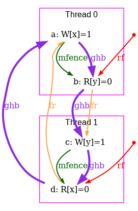
The image above much differs from the one in Sec. 14.2 that describes the same execution and that is reproduced in Fig. 7
Figure 7: The non-SC behaviour of SB is allowed by TSO
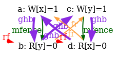
In effect, herd7 can produce three styles of pictures, dot clustered pictures, dot free pictures, and neato pictures with explicit placement of the events of one thread as a column. The style is commanded by the -graph option that accepts three possible arguments: cluster (default), free and columns. The following pictures show the effect of graph styles on the SB example:
| -graph cluster | -graph free | -graph columns |
 |  | 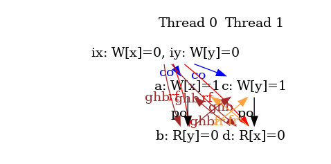
|
Notice that we used another option -squished true that much reduces the information displayed in nodes. Also notice that the first two pictures are formatted by dot, while the rightmost picture is formatted by neato.
One may also observe that the “-graph columns” picture does not look exactly like Fig. 7. For instance the ghb arrows are thicker in the figure. There are many parameters to control neato (and dot), many of which are accessible to herd7 users by the means of appropriate options. We do not intend to describe them all. However, users can reproduce the style of the diagram of this manual using yet another feature of herd7: configuration files that contains settings for herd7 options and that are loaded with the -conf name option. In this manual we mostly used the doc.cfg configuration file. As this file is present in herd7 distribution, users can use the diagram style of this manual:
% herd7 -conf doc.cfg ...
Images are produced or displayed once the model has been executed. As a consequence, forbidden executions won’t appear by default. Consider for instance the test SB+mfences, where the mfence instruction is used to forbid SB non-SC execution. Running herd7 as
% herd7 -model tso-02.cat -conf doc.cfg -show prop -gv SB+mfences.litmus
will produce no picture, as the TSO model forbids the target execution of SB+mfences.
To get a picture, we can run SB+mfences on top of the minimal model, a pre-defined model that allows all executions:
% herd7 -model minimal -conf doc.cfg -show prop -gv SB+mfences.litmus
And we get the picture:
It is worth mentioning again that although the minimal model allows all executions, the final condition selects the displayed picture, as we have specified the -show prop option.
The picture above shows mfence arrows, as all
fence relations are displayed by the minimal model.
However, it does not show the ghb relation, as the minimal
model knows nothing of it.
To display ghb we could write another model file that would be just as
tso-02.cat, with checks erased.
The simulator herd7 provides a simpler technique:
one can instruct herd7 to ignore
either all checks (-through invalid), or a selection of checks
(-skipchecks name1,…,namen).
Thus, either of the following two commands
% herd7 -through invalid -model tso-02.cat -conf doc.cfg -show prop -gv SB+mfences.litmus
% herd7 -skipcheck tso -model tso-02.cat -conf doc.cfg -show prop -gv SB+mfences.litmus
will produce the picture we wish:
Notice that mfence and ghb are displayed because
of the instruction “show mfence ghb” (fence relation are not shown
by default);
while -skipcheck tso works because the tso-02.cat model
names its main check with “as tso”.
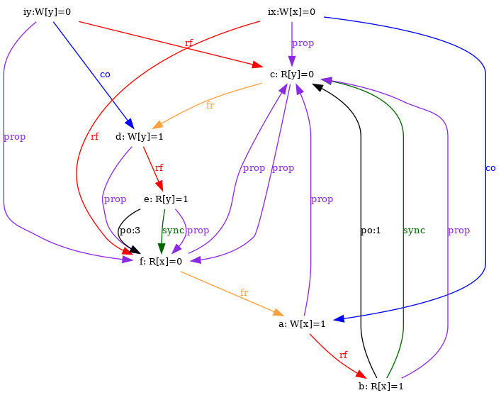
The image above is barely readable.
For such graphs with many relations, the cluster and free modes
are worth a try. The commands:
% herd7 -skipcheck tso -model tso-02.cat -conf doc.cfg -show prop -graph cluster -gv SB+mfences.litmus
% herd7 -skipcheck tso -model tso-02.cat -conf doc.cfg -show prop -graph free -gv SB+mfences.litmus
will produce the images:
 | 
|
Namely, command line options are scanned left-to-right,
so that most of the settings of doc.cfg are kept11
(for instance thick ghb arrows), while the graph mode is overridden.
We describe our cat language for defining models. The syntax of the language is given in BNF-like notation. Terminal symbols are set in typewriter font (like this). Non-terminal symbols are set in italic font (like that). A vertical bar …∣ … denotes alternative. Square brackets […] denote optional components. Curly brackets {…} denotes zero, one or several repetitions of the enclosed components. Parentheses (…) denote grouping.
Model source files may contain comments of the OCaml type
((*…*), can be nested), or line comments starting with
“//” and running until end of line.
The cat language is much inspired by OCaml, featuring immutable bindings, first-class functions, pattern matching, etc. However, cat is a domain specific language, with important differences from OCaml.
There are two structured values: tuples of values and sets of values. One should notice that primitive set of events and structured set of events are not the same thing. In fact, the language prevents the construction of structured set of events. Similarily, there are no structured sets of elements of relations, there are only relations.
A model, or cat program is a sequence of instructions. At startup, pre-defined identifiers are bound to event sets and relations over events. Those pre-defined identifiers describe a candidate execution (in the sense of the memory model). Executing the model means allowing or forbidding that candidate execution.
|
Identifiers are rather standard: they are a sequence of letters, digits, “_” (the underscore character), “.” (the dot character) and “-” (the minus character), starting with a letter. Using the minus character inside identifiers may look a bit surprising. We did so as to allow identifiers such as po-loc.
At startup, pre-defined identifiers are bound to event sets and to relations between events.
Those pre-defined identifiers first describe the events of the candidate execution as various sets, as described by the first table of figure 8.
identifier name description emptyset empty set of events W write events R read events M memory events we have M = W ∪ R IW initial writes feed reads that read from the initial state FW final writes writes that are observed at the end of test execution B branch events RMW read-modify-write events F fence events NAME specific fence events those depend on the test architecture
architecture fence sets X86 MFENCE, SFENCE, LFENCE PPC SYNC, LWSYNC, EIEIO, ISYNC ARM DMB, DMB.ST, DSB, DSB.ST, ISB MIPS SYNC AArch64 DMB.SY, DMB.ST, DMB.ST, …DSB.SY, DSB.ST, DSB.ST, …
Specific fence event sets depend on the test architecture, their name is always uppercase and derives from the mnemonic of the instruction that generates them. The second table of figure 8 shows a (non-exhaustive) list.
Other pre-defined identifiers are relations. Most of those are the program order po and its refinements:
| identifier | name | description | ||
| po | program order | instruction order lifted to events | ||
| addr | address dependency | the address of the second event depends on the value loaded by the first (read) event | ||
| data | data dependency | the value stored by the second (write) event depends on the value loaded by the first (read) event | ||
| ctrl | control dependency | the second event is in a branch controlled by the value loaded by the commfirst (read) event | ||
| rmw | read-exclusive write-exclusive pair | relate the read and write events emitted by matching successful load-reserve store conditional instructions, or atomic rmw instructions. | ||
| amo | atomic modify | relate the read and write events emitted by atomic rmw instructions. | ||
Finally, a few pre-defined relations describe the execution candidate structure and write-to-read communication:
| identifier | name | description | ||
| id | identity | relates each event to itself | ||
| loc | same location | events that touch the same address | ||
| ext | external | events from different threads | ||
| int | internal | events from the same thread | ||
| rf | read-from | links a write w to a read r taking its value from w | ||
Some additional relations are defined by library files written in the cat language, see Sec. 16.7.
Expressions are evaluated by herd7, yielding a value.
|
Simple expressions are the empty relation (keyword 0), identifiers id and tags tag. Identifiers are bound to values, either before the execution (see pre-defined identifiers in Sec. 16.2), or by the model itself. Tags are constants similar to C enum values or OCaml constant constructors. Tags must be declared with the enum instruction. We go back to enum and tags in Sec. 16.4 and 16.4.
Tuples include a constant, the empty tuple (), and constructed tuples ( expr1 , expr1 ,… , exprn), with n ≥ 2. In other words there is no tuple of size one. Syntax ( expr ) denotes grouping and has the same value as expr.
Explicit sets are written as the comma separated list of their elements between curly braces: { expr1 , expr1 ,… , exprn}, with n ≥ 0. Sets are homogenous, in the sense that sets hold elements of the same type.
In case the values exprk are events, the result will be a primitive event set. In case they are elements of relations, the result will be a relation (and not a set of event pairs).
The empty set {} is the empty set of events and the empty relation.
Most operators are overloaded and apply to event sets, relations and explicit sets. However, by nature, some operators apply to relations only (as sequence and transitive closure below) or to sets only (as the cartesian product). Additionally, an event in a context where an event set is expected will be promoted to a singleton event set. The situation of an elementary relation in a relation context is similar.
The transitive and reflexive-transitive closure of an expression are performed by the postfix operators + and *. The postfix operator ^-1 performs relation inversion. The construct expr? (option) evaluates to the union of expr value and of the identity relation. Notice that postfix operators operate on relations only.
There is one prefix operator ~ that performs relation and set complement.
Finally, there is one last unary operator: [expr] that evaluate expr to an event set and returns the identity relation over this set.
Infix operators are | (union), ++ (set addition), ; (sequence), & (intersection), \ (set difference), and * (cartesian product). Infix operators are listed in order of increasing precedence, while postfix and prefix operators bind tighter than infix operators. All infix operators are right-associative, except set difference which is left-associative, and cartesian product which is non-associative.
The union, intersection and difference operators apply to relations and all kinds of sets. The cartesian product takes two event sets as arguments and returns a relation.
The addition operator expr1 ++ expr2 operates on sets: the value of expr2 must be a set of values (or an event, or an element of relation) S and the operator returns the set S augmented with the value of expr1 (or a new event set, or a new relation). By exception, the arguments to the addition operator can also be an elementary relation. It then yields a relation.
For the record, given two relations r1 and r2, the sequence r1; r2 is defined as { (x,y) ∣ ∃ z, (x,z) ∈ r1 ∧ (z,y) ∈ r2}.
Functions calls are written expr1 expr2. That is, functions are of arity one and the application operator is left implicit. Notice that function application binds tighter than all binary operators and looser that postfix operators. Furthermore the implicit application operator is left-associative.
The cat language has call-by-value semantics. That is, the effective parameter expr2 is evaluated before being bound to the function formal parameter(s).
N-ary functions can be encoded either using tuples as arguments or by curryfication (i.e. as functions that return functions). Considering binary functions, in the former case, a function call is written expr1 ( expr2 , expr3); while in the latter case, a function call is written expr1 expr2 expr3 (which by left-associativity, is to be understood as (expr1 expr2) expr3). The two forms of function call are not interchangeable, using one or the other depends on the definition of the function.
Functions are first class values, as reflected by the anonymous function construct fun pat -> expr. A function takes one argument only.
In the case where this argument is a tuple, it may be destructured by the means of a tuple pattern. That is pat above is ( id1 , … idn). For instance here is a function that takes a tuple of relations (or sets) as argument and return their symmetric difference:
fun (a,b) -> (a\b)|(b\a)
Functions have the usual static scoping semantics: variables that appear free in function bodies (expr above) are bound to the value of such free variable at function creation time. As a result one may also write the symmetric difference function as follows:
fun a -> fun b -> (a\b)|(b\a)
The local binding construct let [ rec ] bindings in expr binds the names defined by bindings for evaluating the expression expr. Both non-recursive and recursive bindings are allowed. The function binding id pat = expr is syntactic sugar for id = fun pat -> expr.
The construct
evaluates expr1,…, exprn, and binds the names in the patterns pat1,…, patn to the resulting values. The bindings for pat = expr are as follows: if pat is (), then expr must evaluate to the empty tuple; if pat is id or (id), then id is bound to the value of expr; if pat is a proper tuple pattern (id1,… ,idn) with n ≥ 2, then expr must evaluate to a tuple value of size n (v1,…,vn) and the names id1,…,idn are bound to the values v1,…,vn. By exception, in the case n=2, the expression expr may evaluate to an elementary relation. If so, the value behaves as a tuple of arity two.
The construct
computes the least fixpoint of the equations pat1 = expr1,…, patn = exprn. It then binds the names in the patterns pat1,…, patn to the resulting values. The least fixpoint computation applies to set and relation values, (using inclusion for ordering); and to functions (using the usual definition ordering).
The syntax for pattern matching over tags is:
The value of the match expression is computed as follow: first evaluate expr to some value v, which must be a tag t. Then v is compared with the tags tag1,…,tagn, in that order. If some tag pattern tagi equals t, then the value of the match is the value of the corresponding expression expri. Otherwise, the value of the match is the value of the default expression exprd. As the default clause _ -> exprd is optional, the match construct may fail.
The syntax for pattern matching over sets is:
The value of the match expression is computed as follow: first evaluate expr to some value v, which must be a set of values. If v is the empty set, that the value of the match is the value of the corresponding expression expr1. Otherwise, v is a non-empty set, then let ve be some element in v and vr be the set v minus the element ve. The value of the match is the value of expr2 in a context where id1 is bound to ve and id2 is bound to vr.
The construct also also applies to primitive event sets and relations. If the matched expression is non-empty, then the bound element is an event and an element of relation, respectively. One easily rebuilds an event set (or a relation) for instance by using the singleton construct as { id1 }.
The expression (expr) has the same value as expr. Notice that a parenthesised expression can also be written as begin expr end.
Instruction are executed for their effect. There are three kinds of effects: adding new bindings, checking a condition, and specifying relations that are shown in pictures.
|
The let and let rec constructs bind value names for the rest of model execution. See the subsection on bindings in Section 16.3 for additional information on the syntax and semantics of bindings.
Recursive definitions computes fixpoints of relations. For instance, the following fragment computes the transitive closure of all communication relations:
let com = rf | co | fr
let rec complus = com | (complus ; complus)
Notice that the instruction let complus = (rf|co|fr)+ is equivalent.
Notice that herd7 assumes that recursive definitions are well-formed,
i.e. that they yield an increasing functional.
The result of ill-formed definitions is undefined.
Although herd7 features recursive functions, those cannot be used to compute a transitive closure, due to the lack of some construct say to test relation equality. Nevertheless, one can write a generic transitive closure function by using a local recursive binding:
let tr(r) = let rec t = r | (t;t) in t
Again, notice that the instruction let tr (r) = r+ is equivalent.
Thanks to pattern matching constructs, recursive functions are useful to compute over sets (and tags). For instance here is the definition of a function power that compute power sets:
let rec power S = match S with
|| {} -> { {} }
|| e ++ S ->
    let rec add_e RR = match RR with
    || {} -> { }
    || R ++ RR -> R ++ (e ++ R) ++ add_e RR
    end in
    add_e (power S)
end
The construct
evaluates expr and applies the check check. There are six checks: the three basic acyclicity (keyword acyclic), irreflexivity (keyword irreflexive) and emptyness (keyword empty); and their negations. If the check succeeds, execution goes on. Otherwise, execution stops.
The performance of a check can optionally be named by appending as id after it. The feature permits not to perform some checks at user’s will, thanks to the -skipchecks id command line option.
A check can also be flagged, by prefixing it with the flag
keyword. Flagged checks must be named with the as construct.
Failed flagged checks do not stop execution.
Instead successful flagged checks are recorded under their name,
for herd7 machinery to handle flagged executions later.
Flagged checks are useful for models that define conditions
over executions that impact the semantics of the whole program.
This is typically the case of data races.
Let us assume that some relation race has been defined,
such that an non-empty race relation in some execution
would make the whole program undefined. We would then write:
flag ~empty race as undefined
Then, herd7 will indicate in its output that some
execution have been flagged as undefined.
Procedures are similar to functions except that they have no results: the body of a procedure is a list of instructions and the procedure will be called for the effect of executing those instructions. Intended usage of procedures is to define checks that are executed later. However, the body of a procedure may consist in any kind of instructions. Notice that procedure calls can be named with the as keyword. The intention is to control the performance of procedure calls from the command line, exactly as for checks (see above).
As an example of procedure,
one may define the following uniproc procedure with
no arguments:
procedure uniproc() =
  let com = fr | rf | co in
  acyclic com | po
end
Then one can perform the acyclicity check (see previous section) by executing the instruction:
call uniproc()
As a result the execution will stop if the acyclicity check fails, or continue otherwise.
Procedures are lexically scoped as functions are. Additionally, the bindings performed during the execution of a procedure call are discarded when the procedure returns, all other effects performed (namely flags and shows) are retained.
take (non-empty, comma separated) lists of identifiers as arguments. The show construct adds the present values of identifiers for being shown in pictures. The unshow construct removes the identifiers from shown relations.
The more sophisticated construct
evaluates expr to a relation, which will be shown in pictures with label id. Hence show id can be viewed as a shorthand for show id as id
The forall iteration construct permits the iteration of checks (in fact of any kind of instructions) over a set. Syntax is:
The expression expr must evaluate to a set S. Then, the list of instructions instructions is executed for all bindings of the name id to some element of S. In practice, as failed checks stop execution, this amounts to check the conjunction of the checks performed by instructions for all the elements of S. Similarly to procedure calls, the bindings performed during the execution of an iteration are discarded at iteration ends, all other effects performed are retained.
This construct permits the extension of the current candidate execution by one binding. Syntax is with id from expr. The expression expr is evaluated to a set S. Then the remainder of the model is executed for each choice of element e in S in a context extended by a binding of the name id to e. An example of the construct usage is described in Sec. 14.3.
The construct include "filename" is interpreted as
the inclusion of the model contained in the file whose name is given as
an argument to the include instruction.
In practice, the list of instructions defined by the included model file
are executed.
The string argument is delimited by double quotes “"”,
which, of course, are not part of the filename.
Files are searched according to herd7 rules — see Sec. 17.4.
Inclusion is performed only once. Subsequent include instructions are not executed and a warning is issued.
The conditional instruction allows some control over model execution by setting variants. Variants are predefined tags set on the command line or in configuration files.
The construct if variant "tag" instructions1 else instructions2 end behaves as follows: if the variant tag is set, then the (possibly empty) list of instructions instructions1 is executed, otherwise the (optional, possibly empty) list of instructions instructions2 is executed. If tag is not a recognised variant tag, a warning is issued and the non-existent variant is assumed to be unset.
Users can attain more genericity in their models by defining a bell file, as an addendum, or rather preamble, to a cat file.
The enum construct defines a set of enumerated values or tags. Syntax is
The construct has two main effects. It first defines the tags tag1,…,tagn. Notice that tags do not exist before being defined, that is evaluating the expression tag is an error without a prior enum that defines the tag tag. Tags are typed in the sense that they belong to the tag type id and that tags from different types cannot be members of the same set. The second effect of the construct is to define a set of tags id as the set of all tags listed in the construct. That is, the enum construct performs the binding of id to { tag1,…,tagn}.
Scopes are a special case of enumeration: the construct enum scopes must be used to define hierarchical models such as Nvidia GPUs.
An enum scopes declaration must be paired with two functions narrower and wider that implement the hierarchy amongst scopes. For example:
enum scopes = 'discography || 'I || 'II || 'III || 'IV

let narrower(t) = match t with
  || 'discography -> {'I, 'II, 'III, 'IV}
end

let wider(t) = match t with
  || 'I -> 'discography
  || 'II -> 'discography
  || 'III -> 'discography
  || 'IV -> 'discography
end
Here we define five scopes, where the first one, discography, is wider than all the other ones.
The predefined sets of events W, R, RMW, F, and B can be annotated with user-defined tags (see Sec. 16.4).
The construct :
takes the identifier of a pre-defined set and a possibly empty, square bracketed list of tags.
The primitive tag2instrs yields, given a tag ’t, the set of instructions bearing the annotation t that was previously declared in an enumeration type.
The primitive tag2scope yields, given a tag ’t, the relation between instructions TODO
|
A model is a list of instructions preceded by an optional architecture
specification and an optional comment.
Architecture specification is a name that follows herd7 conventions for identifiers. Identifiers that are not valid architecture names, such as AArch64, PPC etc., are silently ignored.
The following model-comment can be either a name or a string enclosed in double quotes “"”.
If only one name is present, it will act both as tentative architecture specification and as a comment.
When present, model architecture specifications will be checked against test architectures, see also option -archcheck.
Models operate on candidate executions (see Sec. 16.2), instructions are executed in sequence, until one instruction stops, or until the end of the instruction list. In that latter case, the model accepts the execution. The accepted execution is then passed over to the rest of herd7 engine, in order to collect final states of locations and to display pictures. Notice that the model-comment will appear in those picture legends.
TODO:
The standard library is a cat file stdlib.cat which all models include by default. It defines a few convenient relations that are thus available to all models.
| identifier | name | description | ||
| po-loc | po restricted to the same address | events are in po and touch the same address, namely po ∩ loc | ||
| rfe | external read-from | read-from by different threads, namely rf ∩ ext | ||
| rfi | internal read-from | read-from by the same thread, namely rf ∩ int | ||
For most models, a complete list of communication relations would also include co and fr. Those can be defined by including the file cos.cat (see Sec. 14.4).
| identifier | name | description | ||
| co | coherence | total strict order over writes to the same address | ||
| fr | from-read | links a read r to a write w′ co-after the write w from which r takes its value | ||
| coi, fri | internal communications | communication between events of the same thread | ||
| coe, fre | external communications | communication between events of different threads | ||
Notice that the internal and external sub-relations of co and fr are also defined.
Fence relations denote the presence of a specific fence (or barrier) in-between two events. Those can be defined by including architecture specific files.
| file | relations | |
| x86fences.cat | mfence, sfence, lfence | |
| ppcfences.cat | sync, lwsync, eieio, isync, ctrlisync | |
| armfences.cat | dsb, dmb, dsb.st, dmb.st, isb, ctrlisb | |
| mipsfences.cat | sync | |
| aarch64fences.cat | … | |
In other words, models for, say, ARM machines should include the following instruction:
include "armfences.cat"
Notice that for the Power (PPC) (resp. ARM) architecture, an additional relation ctrlisync (res. ctrlisb) is defined. The relation ctrlisync reads control +isync. It means that the branch to the instruction that generates the second event additionally contains a isync fence preceding that instruction. For reference, here is a possible definition of ctrlisync:
let ctrlisync = ctrl & (_ * ISYNC); po
One may define all fence relations by including the file fences.cat. As a result, fence relations that are relevant to the architecture of the test being simulated are properly defined, while irrelevant fence relations are the empty relation. This feature proves convenient for writing generic models that apply to several concrete architectures.
The command herd7 handles its arguments like litmus7. That is, herd7 interprets its argument as file names. Those files are either a single litmus test when having extension .litmus, or a list of file names when prefixed by @.
There are many command line options. We describe the more useful ones:
The main purpose of herd7 is to run tests on top of memory models. For a given test, herd7 performs a three stage process:
We now describe options that control those three stages.
In fact, herd7 accepts potentially infinitely many models, as models can be given in text files in an adhoc language described in Sec. 16. The herd7 distribution includes several such models: minimal.cat and uniproc.cat are the text file versions of the homonymous internal models, but may produce pictures that show different relations. The herd7 distribution also includes models for a variety of architectures and several models for the C language. Model files are searched according to the same rules as configuration files. Some architectures have a default model: arm.cat model for ARM, ppc.cat model for PPC, x86tso.cat for X86, and aarch64.cat for AArch64 (ARMv8).
exists p, ~exists p, or forall p.
The semantics of recognised tags is as follows:
exists and forall, and false
for ~exists.
exists and ~exists,
and false for forall.
Those options intentionally omit some of the final states that herd7 would normally generate.
exists p is validated, and as soon as a condition ~exists p or
forall p is invalidated. Default is false.<int> pictures have been collected. Default is to
collect all (specified, see option -show) pictures.
These options control the content of DOT images.
We first describe options that act at the general level.
\myth{n}. Assembler instructions are locations in nodes
are argument to an \asm command. It user responsability to define
those commands in their LATEX documents that include the pictures.
Possible definitions are \newcommand{\myth}[1]{Thread~#1}
and \newcommand{\asm}[1]{\texttt{#1}}.
Default is false.
A few options control picture legends.
exists,
kind Forbid being ~exists,
and kind Require being forall.
Default is false.
A few options control what is shown in nodes and on their sizes, i.e. on how events are pictured.
Then we list options that offer some control on which edges are shown.
We recall that the main controls over the shown and unshown edges are
the show and unshow directives in model definitions —
see Sec. 16.4.
However, some edges can be controlled only with options (or configuration
files) and the -unshow option proves convenient.
show directive in model definition and any -doshow command
line option.
Other options offer some control over some of the attributes defined in Graphviz software documentation. Notice that the controlled attributes are omitted from DOT files when no setting is present. For instance in the absence of a -spline <tag> option, herd7 will generate no definition for the splines attribute thus resorting to DOT tools defaults. Most of the following options accept the none argument that restores their default behaviour.
Those options are the same as the ones of litmus7 — see Sec. 4.
exists,
kind Forbid being ~exists
and kind Require being forall.
The syntax of configuration files is minimal: lines “key arg” are interpreted as setting the value of parameter key to arg. Each parameter has a corresponding option, usually -key, except for the single letter option -v whose parameter is verbose.
As command line option are processed left-to-right, settings from a configuration file (option -conf) can be overridden by a later command line option. Configuration files will be used mostly for controling pictures. Some configuration files are are present in the distribution. As an example, here is the configuration file apoil.cfg, which can be used to display images in free mode.
#Main graph mode
graph free
#Show memory events only
showevents memory
#Minimal information in nodes
squished true
#Do not show a legend at all
showlegend false
The configuration above is commented with line comments that starts
with “#”.
The above configuration file comes handy to eye-proof model output,
even for relatively complex tests, such as IRIW+lwsyncs
and IRIW+syncs:
% herd7 -conf apoil.cfg -show prop -doshow prop -gv IRIW+lwsyncs.litmus
% herd7 -through invalid -conf apoil.cfg -show prop -doshow prop -gv IRIW+syncs.litmus
In the command lines above, -show prop instructs herd7 to produce images of the executions that validate the final test condition, while -doshow prop instructs herd7 to display the relation named “prop”. In spite of the unfortunate name clashes, those are not to be confused…
We run the two tests on top of the default Power model that computes, amongst others, a prop relation. The model rejects executions with a cyclic prop. One can then see that the relation prop is acyclic for IRIW+lwsyncs and cyclic for IRIW+syncs:
Notice that we used the option -through invalid in the case of IRIW+syncs as we would otherwise have no image.
Configuration and model files are searched first in the current directory; then in the search path; then in any directory specified by setting the shell environment variable HERDLIB; and then in herd installation directory, which is defined while compiling herd7.